The team shipped a fix on Monday and, two weeks later, activation was up 2 points. The dashboard turns green and the meeting becomes a celebration. But in those two weeks there was also a campaign, and more large accounts signed up. Did the fix work? Nobody can say.
Comparing before and after is the most common way to assess a change, and one of the least reliable, because many things change at once. Hypothesis testing organizes the question so the result says something about the cause.
What a hypothesis test is
A hypothesis test turns an assumption about a cause, a behavior or a result into a claim the data can contradict. The term joins two different things:
- The product hypothesis: an idea about what will happen and why.
- The statistical test: a procedure for assessing whether an observed difference is compatible with chance. It comes from the work of Ronald Fisher and of Jerzy Neyman and Egon Pearson, in the early 20th century.
In digital products, the best-known form is the A/B test, or controlled experiment: randomly assigned groups get different versions at the same time. Randomization is what matters, because campaigns, seasonality and customer types tend to spread evenly across the groups (Kohavi, Tang & Xu, 2020).
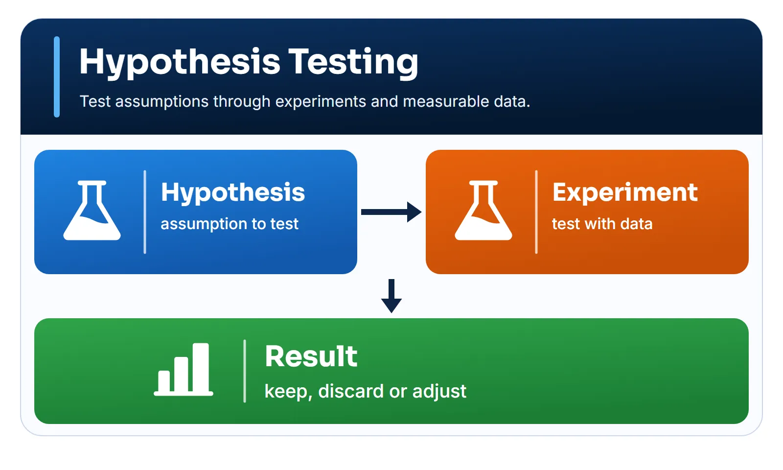
What makes a hypothesis testable
A good sentence template is: if we do [change], [metric] will [direction and size] for [audience] within [timeframe], because [mechanism]. The mechanism matters: it’s what shows what to learn if the result comes out differently.
| Vague | Testable |
|---|---|
| The assistant will improve | 7-day activation rises 4 points |
| Users will like it | 30-day retention doesn’t fall |
| It should convert more | Sign-up rises from 10% to 12.5% |
25% of what?
“A freemium offer will increase sign-ups by 25%” sounds clear, but it has two readings. Starting from 10%:
- 25% relative: from 10% to 12.5%, a gain of 2.5 percentage points.
- 25 percentage points: from 10% to 35%.
The difference isn’t just vocabulary. With the usual parameters explained below, detecting the first takes about 2,504 people per group. The second, about 40.
When to use it and when to avoid it
When to use it
- Product, UX and conversion changes with enough traffic
- Assessing AI features in real use
- Operational improvements with comparable groups
- When the decision is costly and the doubt is real
When to avoid it
- Too little volume to detect a relevant effect
- Mandatory security or legal fixes
- When groups affect each other, as in a market with shared supply
- When the decision is already made, whatever the result
How to apply it
- Write the hypothesis. Include change, metric, audience, timeframe and mechanism.
- Define the primary metric and the unit. Choose one metric to decide on and state what gets randomized: user, account or store.
- Define the guardrails. These are the metrics that can’t get worse, such as retention, cost and security.
- Calculate the sample. Choose the smallest effect that justifies the change and calculate how many cases you need.
- Record the decision rule. Write down in advance what will lead you to ship, revert or repeat.
- Run to the end. Don’t stop the test because the result looks good. Check that the group split came out as planned.
- Read and decide. Look at the effect and its interval, the guardrails and the recorded rule.
The primary metric is the most important decision in step 2. It must be tied to customer value, react within the test’s timeframe and be hard to inflate. Button clicks react fast, but they rise even with a confusing interface. Annual revenue is what counts, but it takes too long to respond. A good metric sits in the middle. Kohavi, Tang and Xu speak of an overall evaluation criterion: the metric, or combination of metrics, that sums up the experiment’s goal. Use just one to decide, and leave the others to explain the result.
Worked example: recovering activation
After an AI assistant launched, a SaaS product’s activation fell from 40% to 30%. An activated account is one that saves or shares its first result within 7 days. The investigation pointed to two likely causes: the data index was built on the first request, which made the first generation slow, and the assistant opened empty, with no suggestions.
These are good hypotheses, but they’re still hypotheses. The working hypothesis: if we index data right after connection and bring back the suggestions, 7-day activation of new accounts will rise at least 4 points, because fewer accounts will abandon the first generation.
| Item | Definition |
|---|---|
| Unit | Account |
| Audience | New accounts |
| Split | 50/50, randomized at sign-up |
| Primary metric | 7-day activation |
| Current rate | 30% |
| Minimum effect | +4 points |
The unit is the account, because users of the same account share data and couldn’t see different versions. Testing both fixes together is also a choice: the test answers whether the package works, not which part does.
In statistical language, the null hypothesis (H0) says the two groups’ rates are equal, and the alternative (H1) says they differ. The test doesn’t try to prove H1. It assesses how surprising the data would be if H0 were true.
Guardrails
A change can improve the primary metric and hurt the business. So the team sets limits on what can’t get worse. Kohavi, Tang and Xu separate the guardrails that protect the business from those that protect trust in the experiment itself, such as checking the group split.
| Guardrail | Limit |
|---|---|
| 30-day retention | Drop of up to 1 point |
| Indexing cost | Up to 0.50 more per account |
| Security incidents | None |
Sample size
Every test lives with two possible errors:
| Decision | No effect | Real effect |
|---|---|---|
| Ship | False positive | Correct |
| Don’t ship | Correct | False negative |
Significance is the accepted risk of a false positive. Power is the chance of detecting a real effect, that is, of avoiding a false negative. To compare two proportions, with 5% two-sided significance and 80% power, the approximate math is this:
- Accounts per group
- 1.96: for 5% significance
- 0.84: for 80% power
- Sum of the two rates' variances
- Minimum effect, as a proportion
With 30% and 34%:
- S = 0.30 × 0.70 + 0.34 × 0.66 = 0.4344
- d = 0.04, so d² = 0.0016
- (1.96 + 0.84)², with the full values, comes to 7.85
- n = 7.85 × 0.4344 ÷ 0.0016 = 2,131 accounts per group
Because d is squared, the minimum effect dominates the math. With 600 new accounts a week across both groups:
| Effect | Per group | Weeks |
|---|---|---|
| 2 points | 8,391 | 28 |
| 4 points | 2,131 | 7.1 |
| 6 points | 961 | 3.2 |
| 10 points | 354 | 1.2 |
Choosing the minimum effect is a business decision, not a statistical one. The team settles on 4 points, because less wouldn’t pay for keeping the indexing. The test runs for eight full weeks, to cover weekly cycles, and each account gets another 7 days to mature.
Decision rule, recorded in advance: ship if the 95% interval for the difference sits entirely above zero and no guardrail breaks. If the interval includes zero, the result is inconclusive.
Result
Each group had 2,400 accounts:
| Group | Activated | Rate |
|---|---|---|
| Control | 724 | 30.2% |
| Treatment | 828 | 34.5% |
The difference is 4.3 percentage points, or 14.4% in relative terms. The 95% interval runs from 1.7 to 7.0 points, with z = 3.21 and a p-value of 0.0013.
In the right order, the reading is:
- The split came out as planned. This is the first check. With 4,800 accounts, a split of 2,520 and 2,280 would have less than a 0.1% chance of occurring by accident and would point to a randomization problem. In that case, no other number would deserve trust until the cause turned up.
- The p-value is low. If there were no effect, a difference this large or larger would appear in about 1 of every 750 experiments. That doesn’t mean a 99.9% chance the fix works.
- The interval matters more. The data are compatible with gains of 1.7 to 7.0 points. There’s a sign of an effect, but its size is uncertain, and part of the interval falls below the desired 4 points.
- The guardrails passed, with one caveat. Cost rose by 0.38, and there were no incidents. 30-day retention went from 61.8% to 61.5%, but the interval for that difference runs from −3.1 to +2.5 points. The test doesn’t have the sample to guarantee the 1-point limit, so retention stays monitored after launch.
The team ships the fix. It recovers about 4 of the 10 lost points, and the test also shows what it didn’t solve: nearly 6 points are still missing, and the next cycle starts there.
How not to fool yourself with the result
Many experiment errors happen in the reading.
- Peeking and stopping early. Looking at the result every week and stopping at the first “significant” one increases false positives. In a simulation run for this article, with 300,000 tests with no real effect, looking only at the end gave 4.9% false positives. Looking at each of the 8 weeks gave 17.6%. If the team needs to monitor the test, there are methods designed for that (Johari et al., 2017).
- Testing many things. With 10 independent comparisons at 5%, the chance of at least one false positive is 40%. With 20, it’s 64%. A segment that “won” should become a new hypothesis, not a conclusion.
- Reading “not significant” as “doesn’t work”. Large effects can go unnoticed in small samples (Greenland et al., 2016).
- Reading “significant” as “important”. With a large sample, a trivial effect is significant too. The p-value doesn’t measure the size of the effect.
- Treating the interval as a certainty. The 95% describes the method over many repetitions. A specific interval either contains the true value or doesn’t.
- Moving the goalposts. Changing the primary metric after seeing the data invalidates the decision rule.
- Believing the surprising number too much. A result that’s too large, or too good, is often a sign of an instrumentation error. Check the data before celebrating.
The American Statistical Association’s statement on p-values captures the spirit well: a p-value doesn’t measure the probability that a hypothesis is true, decisions shouldn’t rest on a threshold alone, and proper inference requires transparency about what was analyzed (Wasserstein & Lazar, 2016).
When an A/B test isn’t possible
Many B2B products have few accounts. In the table above, with 600 accounts a week, detecting 2 points would take more than half a year, and with less traffic the test becomes unfeasible. In those cases, a team can look for a larger effect, test a metric closer to the change, roll out in stages, comparing groups that get the change at different times, or use qualitative research. These are weaker forms of evidence, and the decision should say so.
How to use an LLM
An LLM helps turn an idea into a protocol: it drafts the hypothesis, suggests guardrails and points out biases. It can get the form right and the math wrong, so recalculate everything in a reliable tool. And remember: AI helps with the design, but it doesn’t produce evidence by drafting a hypothesis. Evidence comes from the experiment.
Act as a product experimentation specialist.Business hypothesis: [statement].Current metric and baseline: [data].Proposed change: [intervention].Audience, experimental unit and constraints: [describe].
Turn the idea into a measurable hypothesis, including H0/H1 when it makessense. Define the primary metric, guardrails, success criteria, segments,bias risks and experimental design (A/B or an alternative). Explain whatinformation is needed to estimate sample size and duration. Don't declaresignificance, statistical power or causal gain without sufficient data.
Expected output: an experiment protocol and analysis plan.
Before trusting the answer:
- Redo the sample math. Use a calculator or a script, and check whether the effect is relative or in points.
- Check the unit. Ask whether the randomized unit is the same as the metric’s.
- Ask what would invalidate the test. The model should point out interference between groups, seasonality and randomization failures.
- Sanitize the context. Don’t send individual customer data or identifiable internal metrics.
Combine it with other frameworks
- MECE principle: defines stages and metrics without overlap.
- Fishbone diagram: generates hypotheses about causes.
- 5 Whys: digs into a cause before testing the fix.
- Decision matrix: chooses which intervention is worth testing.
- OODA loop: uses the result to orient the next cycle.
References
- Greenland, S., Senn, S. J., Rothman, K. J., Carlin, J. B., Poole, C., Goodman, S. N. & Altman, D. G. (2016). Statistical tests, P values, confidence intervals, and power: a guide to misinterpretations. European Journal of Epidemiology, 31(4), 337–350. DOI
- Johari, R., Koomen, P., Pekelis, L. & Walsh, D. (2017). Peeking at A/B Tests: Why It Matters, and What to Do About It. KDD ‘17, 1517–1525. DOI
- Kohavi, R., Tang, D. & Xu, Y. (2020). Trustworthy Online Controlled Experiments. Cambridge University Press. DOI
- Wasserstein, R. L. & Lazar, N. A. (2016). The ASA Statement on p-Values: Context, Process, and Purpose. The American Statistician, 70(2), 129–133. DOI