Build or buy? The vendor’s proposal shows the annual license, and the internal estimate shows development. Each side tells part of the story, and the two numbers end up compared as if they were the same thing.
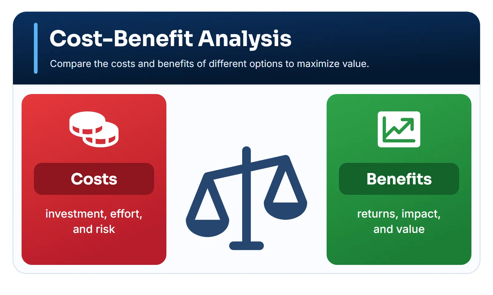
Cost-benefit analysis puts the alternatives on the same basis: same horizon, same currency, all costs and all benefits, year by year. The result is a number, but the bigger gain lies elsewhere: the analysis exposes the assumptions that must be true for that number to hold.
What it is
The analysis compares each alternative’s costs and benefits over a defined period, taking into account when each amount occurs. Whatever can’t be safely converted into money goes in separately, as information for the decision.
The technique was born in the appraisal of public works. Its proposal is attributed to the French engineer Jules Dupuit in 1844, and it gained scale in the United States with the Flood Control Act of 1936, which conditioned projects on benefits exceeding costs (Britannica). Governments still have their own guides, such as the UK’s Green Book and the US Circular A-94.
In companies, the same logic shows up in business cases, with one important difference: the perspective is the organization’s, not society’s. That changes the discount rate and the effects considered.
When to use it and when to avoid it
When to use it
- Building or buying a system
- Modernization, automation and migration
- Investments with costs and gains spread over time
- When someone needs to approve a budget
When to avoid it
- When the main effects can't be estimated
- In small decisions, where the analysis costs more than the mistake
- When a legal or ethical requirement allows no trade-off
- When non-financial criteria dominate: use a decision matrix
How to do it, step by step
- Define the alternatives and the horizon. Use the same period for all and include keeping the current situation, when that’s a real option.
- List the full costs. Include implementation, migration, operation, training, security and exit.
- List the benefits and how to measure them. Prefer observable effects, such as revenue, retention or avoided cost.
- Build the period-by-period flow. Use constant or nominal values, without mixing them.
- Calculate the indicators. Keep the discount rate explicit.
- Test sensitivity. Vary the main assumptions and record intangibles separately.
The indicators
Each indicator answers a question. Used together, they complement each other.
| Indicator | Question | Limit |
|---|---|---|
| TCO | How much does it cost over time? | Ignores benefits |
| NPV | How much net value, in today’s money? | Depends on the rate |
| ROI | How much comes back per unit invested? | Ignores time and scale |
| Payback | How long until I recover the investment? | Ignores what comes after |
NPV is the central indicator, because it considers the whole flow and when each amount occurs:
- Benefits in period t
- Costs in period t
- Discount rate per period
- Last period of the horizon
How to choose the discount rate
The rate represents the opportunity cost: the return the money would earn in its best alternative use. In companies, it usually comes from finance, as a hurdle rate or the cost of capital. The higher it is, the more it favors quick gains and penalizes projects with distant returns. Three precautions avoid most problems:
- Set it before calculating. A rate chosen after seeing the result is just a convenient adjustment.
- Match the rate to the value basis. Constant and nominal values can’t be mixed in the same analysis. Flows in today’s money call for a real rate, and flows with inflation built in call for a nominal rate (OMB, 1992).
- Say whether there’s a risk premium. If the rate already embeds risk, treating the same risk in scenarios means counting it twice.
Worked example: building or buying a CRM
A company compares two options over a five-year horizon:
- Option A, build: 1,000 of development in year 0 and 280 per year for maintenance, infrastructure and security. Benefits of 300 in year 1, because the system goes live mid-year, and 800 per year after that, thanks to tailored processes.
- Option B, buy: 300 of implementation and migration in year 0 and 360 per year for licenses and administration. Benefits of 450 in year 1 and 650 per year after that.
| Year | A: net | B: net | A: cumulative | B: cumulative |
|---|---|---|---|---|
| 0 | −1,000 | −300 | −1,000 | −300 |
| 1 | 20 | 90 | −980 | −210 |
| 2 | 520 | 290 | −460 | 80 |
| 3 | 520 | 290 | 60 | 370 |
| 4 | 520 | 290 | 580 | 660 |
| 5 | 520 | 290 | 1,100 | 950 |
At a real rate of 12% per year, set by the company as its opportunity cost, the indicators are:
| Indicator | A | B | Best |
|---|---|---|---|
| 5-year TCO | 2,400 | 2,100 | B |
| Net, undiscounted | 1,100 | 950 | A |
| Simple ROI | 46% | 45% | Tie |
| Payback | Year 3 | Year 2 | B |
| NPV at 12% | 428 | 567 | B |
Undiscounted, A wins by 150. Discounted, B wins by 139. Looking only at ROI would give a tie, and looking only at the net figure would pick the wrong option at this rate.
Where the reversal comes from
Each year’s discount factor is . At 12%, an amount received in year 5 is worth 0.57 of the same amount today.
| Year | Factor | A discounted | B discounted |
|---|---|---|---|
| 0 | 1.000 | −1,000.0 | −300.0 |
| 1 | 0.893 | 17.9 | 80.4 |
| 2 | 0.797 | 414.5 | 231.2 |
| 3 | 0.712 | 370.1 | 206.4 |
| 4 | 0.636 | 330.5 | 184.3 |
| 5 | 0.567 | 295.1 | 164.6 |
| NPV | 428 | 567 |
Option A requires 700 more right at the start, when the factor is 1, and only makes up the difference in the final years, when each unit is worth less. The 520 from year 5 becomes 295. That’s the effect a simple sum doesn’t show.
def npv(flows, rate):    return sum(f / (1 + rate) ** t for t, f in enumerate(flows))
a = [-1000, 20, 520, 520, 520, 520]b = [-300, 90, 290, 290, 290, 290]
print(round(npv(a, 0.12)), round(npv(b, 0.12)))  # 428 567print(round(npv(a, 0.05)), round(npv(b, 0.05)))  # 775 765
Sensitivity
The question now is what would have to change for the answer to change.
| Scenario | A’s NPV | B’s NPV | Best |
|---|---|---|---|
| Base (12%, 5 years) | 428 | 567 | B |
| 5% rate | 775 | 765 | A, narrowly |
| 7-year horizon | 927 | 845 | A |
| Development 30% more expensive | 128 | 567 | B |
| A’s benefits 20% lower | −59 | 567 | B |
| B’s annual cost 30% higher | 428 | 177 | A |
| B’s benefits 20% lower | 428 | 134 | A |
Three assumptions hold the decision up:
- Useful life: at a 12% rate, the advantage moves to A between the sixth and seventh year. The question is how long the system will stay useful without a rewrite.
- Price increases: if B’s annual cost rises by about 11%, from 360 to around 400, the options tie. A price adjustment clause in the contract is worth as much as the initial price.
- A’s extra benefit: this is the weakest estimate, because A only pays off if the extra 150 per year is real. With benefits 20% lower, A’s NPV turns negative.
What stays out of the math
Some effects matter and have no reliable value. Circular A-94’s guidance is to list all effects, even without a monetary value, and to quantify what is possible in physical measures. In this case:
- Roadmap control: A lets the company prioritize what it needs, without depending on the vendor.
- Dependency: B creates an exit cost. A creates a dependency on whoever knows the code.
- Security and compliance: with A, the responsibility is entirely internal. With B, part of it is shared and must be verified.
Assigning an invented value to these items would only give an appearance of precision. They sit beside the number, in the decision conversation.
The example’s recommendation: buy B, negotiating a contractual limit on price increases and easy data export. The decision should be revisited if the expected horizon goes beyond seven years or if a pilot shows A’s extra benefit is real.
Optimistic estimates
The analysis inherits the biases of whoever does the estimating. The UK government recognizes this to the point of keeping a supplementary guide on optimism bias, which directs adjustments to cost and time estimates when robust primary evidence is lacking.
Flyvbjerg (2008) separates optimism bias, which is involuntary, from strategic misrepresentation, which is deliberate: inflating benefits to get a project approved. To address both, he proposes reference class forecasting: instead of estimating from the project’s own plan, look at the actual performance of comparable projects.
In practice, the question is how much similar projects cost and how long they took, inside or outside the company. In the example, if the last internal systems cost 30% more than planned, the “development 30% more expensive” row stops being a bad scenario and becomes the base case.
Common mistakes
- Different horizons: comparing three years of one option with five of another.
- Half the costs: counting the license and forgetting migration and training, or counting development and forgetting maintenance.
- Hours as a benefit: saving a thousand hours only becomes value if that time goes into something that produces results.
- Double counting: recording the same gain as both productivity and cost reduction.
- Comparing with nothing: ignoring what would happen without the project, which is the real baseline.
How to use an LLM
An LLM helps recall forgotten cost categories, build the structure of the flow and propose sensitivity scenarios. It doesn’t know your prices, and figures cited from memory may be wrong or outdated. Do the final calculations in a spreadsheet or script.
Run a cost-benefit analysis between [option A] and [option B].Horizon: [years].Known upfront and recurring costs: [data].Known quantifiable benefits: [data].Qualitative benefits: [list].Discount rate, if applicable: [value or "not set"].Value basis: [constant or nominal].
Build the period-by-period flow of costs and benefits, state theassumptions and separate estimated values from proven ones. Point outcost categories that seem to be missing.
Calculate the appropriate indicators (total cost, net benefit, ROI,payback and NPV, when the data allows). Include scenarios and sensitivityanalysis, and say which assumptions would change the recommendation.
Don't invent prices or arbitrarily monetize intangible gains.
Expected output: a comparative economic table, assumptions, risks and tipping points.
Before trusting the answer:
- Redo the math. Copy the flow into a spreadsheet and recalculate the indicators.
- Check every number. Separate what came from your data from what the model suggested.
- Look for missing costs. Ask what happens at the end of the contract or the system’s useful life.
- Sanitize the context. Proposals and financial data are usually confidential.
Combine it with other frameworks
- Decision matrix: brings together the financial result and criteria that don’t fit the math, such as security and vendor dependency.
- Scenario planning: tests the decision under coherent futures, beyond varying one assumption at a time.
- Pre-mortem analysis: helps find costs and risks left out of the spreadsheet.
- Hypothesis testing: validates the most uncertain benefit with a pilot.
References
- Boardman, A. E., Greenberg, D. H., Vining, A. R. & Weimer, D. L. (2018). Cost-Benefit Analysis: Concepts and Practice (5th ed.). Cambridge University Press.
- Office of Management and Budget (1992). Circular A-94: Guidelines and Discount Rates for Benefit-Cost Analysis of Federal Programs. Link
- HM Treasury. The Green Book. Link
- HM Treasury. Green Book supplementary guidance: optimism bias. Link
- Flyvbjerg, B. (2008). Curbing Optimism Bias and Strategic Misrepresentation in Planning: Reference Class Forecasting in Practice. European Planning Studies, 16(1), 3–21. DOI
- Encyclopaedia Britannica. Cost-benefit analysis. Link